3. 课后练习-图像处理

课后练习2

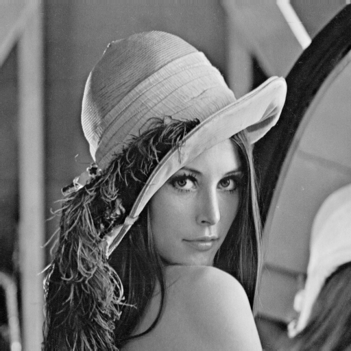
Required libs:Numpy PIL Scipy Matplotlib cv2 ## Q1. Write a python script to open the “lena.png” file using opencv.

• Display the opened image in a new window named “Display Lena”
• Save the image to a new file named “lena_resaved.png”
  
  

  import cv2 as cv
  img = cv.imread("lena.png") # cv2.imread('path')  read the img
  cv.imshow("Display Lena",img) #cv2.imshow(windowname,path)
  cv.waitKey(0) #to let the window display until clicking/pressing
  cv.imwrite("lena_resaved.png",img) #cv2.imwrite(filename,path,params)

Q2. Use PIL and Matplotlib libraries for Q2.

Use “lena.png” to perform following operations and save the images:

• Crop a section from the image whose vertices are (100,100), (100,400), (400,100), (400,400).
  (hint: convert the cv2 image into PIL Image)
  
• Rotate the cropped image by 45 degrees counter-clockwise.
• Perform histogram equalization on lena.png. (hint: use ImageOps.equalize from PIL)
• Use matplotlib to plot the histogram figure for both original image and processed image.
  (hint: use histogram() function in PIL)
  
• Perform Max Filtering, Min Filtering, and Median Filter on lena.png. (hint: PIL.ImageFilter)
  
• Perform Gaussian Blur with sigma equal to 3 and 5. (hint: PIL.ImageFilter)
  

  import cv2
  from PIL import Image 
  from PIL import ImageOps 
  from PIL import ImageFilter as filter
  from matplotlib import pyplot as plt  
  
  pil_img=Image.open("lena.png") #open img in pil 
  #(in cv2 lib, img is opened as array)
  # load cv img: Image.fromarray()
  pil_img.show() # show the img
  img_crop = pil_img.crop((100,100,300,300)) #crop((start point,hight,width))
  img_crop.show() #show the img
  
  img_rota = img_crop.rotate(45) #rotate(degree)
  img_rota.show()
  
  img_eql=ImageOps.equalize(pil_img) 
  #ImageOps.equalize(path) histogram equalize the imge
  
  plt.plot(range(0,256),img_eql.histogram()) 
  #pyplot(aix,img) plot someting   
  #img.histogram()  return the histogram
  plt.show()
  plt.show(rang(0,256),pil_img.histogram())
  plt.show()  
  
  img_max = pil_img.filter(filter.maxfilter()) 
  #filter.(Imagefilter.parm()) add filters
  img_max.show()
  
  img_min=pil_img.filter(filter.minfilter())
  img_min.show()
  
  img_mid=pil_img.filter(filter.medianfilter())
  img_mid.show()
  
  
  img_gus3=pil_img.filter(filter.gaussianblur(radius=3))
  img_gus3.show()
  
  img_gus10=pil_img.filter(filter.gaussianblur(radius=10))
  img_gus10.show()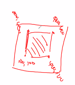

  

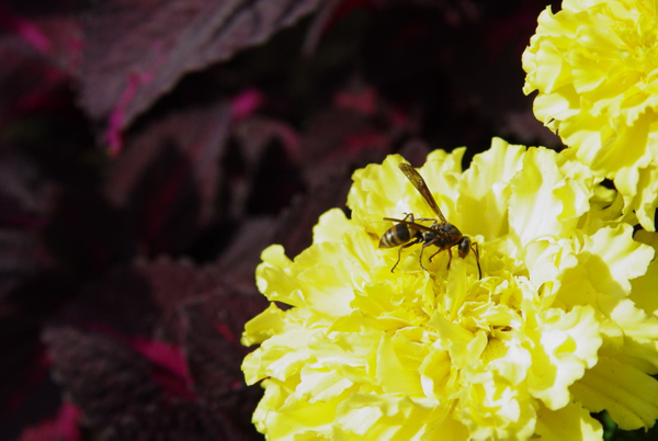
Q3. Colour space conversion. Use Python OpenCV functions to perform following operations on

“bee.png” and save the images at each step.

• Read the image.
• Convert the image to HSV(Hu Satuation Value:包含了三个通道：单色(H)，饱和度(S)，灰度(V)) color space.
• Perform histogram equalization on V channel by cv2.equalizeHist().
• Convert the result image to BGR color space.
• Show the image by cv2.imshow() and save the image.

  import cv2
  from PIL import ImageOps 
  from PIL import ImageFilter as filter
  
  bee_img = cv2.imread("bee.png")
  bee_hsv = cv2.cvtColor(bee_img,cv2.COLOR_BGR2HSV)
  bee_hsv.imshow()
  
  bee_hsv[:,:,2]= cv2.equalizeHist(bee_hsv[:,:,2])
  # 2 presents the channel 2: V
  bee_rgb = cv2.cvtColor(bee_hsv,cv2.COLOR_HSV2BGR)
  cv2.imshow("norm",bee_rgb)
  
  bee_img[:,:,2]= cv2.equalizeHist(bee_rgb[:,:,2])
  bee_img = cv2.cvtColor(bee_hsv,cv2.COLOR_HSV2BGR)
  cv2.imshow("rgb",bee_img)